Template-Space Projection

While data is shared in a subject’s own T1w space, it is possible to move the maps onto a shared template, making them ready for group-level comparison.

Two routes share the same to_template entry point:

The volume route lands on MNI305 via the linear affine FreeSurfer fits during recon-all (stored under the historical name talairach.lta).

The surface route walks the volume through vol_to_surf onto the subject’s fsnative mesh, then resamples onto fsaverage.

Both routes accept single maps, batched (n_trials, n_voxels) arrays, and fsnative-surface arrays.

Note

Run plot_01 first so the shared data directory has the FreeSurfer recon and anatomical mask this example reads. Install the template extras with uv sync --extra template or pip install "laion-fmri[template]".

Bind the shared data directory and load one subject

Plot_01 populated the quickstart directory with the FreeSurfer recon and anatomical mask that the projection chain reads. Pick up the same directory here and load one subject.

import os

from laion_fmri.config import dataset_initialize
from laion_fmri.subject import load_subject

# define and initialize the data directory
data_dir = os.environ.get(
    "LAION_FMRI_EXAMPLE_DATA_DIR",
    os.path.join(os.getcwd(), "laion_fmri_quickstart"),
)
os.makedirs(data_dir, exist_ok=True)
dataset_initialize(data_dir)

# set subject information
subject_id = "sub-01"
session = "ses-01"
roi = "FFA1"

# load and inspect the subject
sub = load_subject(subject_id)
print(f"Subject:        {sub.subject_id}")
print(f"FS recon ready: {sub.has_freesurfer()}")
print(f"Anatomical:     {sub.has_anatomical()}")

Subject:        sub-01
FS recon ready: True
Anatomical:     True

Pick a per-voxel map to project

Anything that has one value per brain-mask voxel can travel through the projection. A session-level noise-ceiling map is a convenient starting point but mean betas, decoding accuracies, or any other per-voxel summary slot in the same way.

import numpy as np

nc = sub.get_noise_ceiling(session=session)
print(f"NC shape:    {nc.shape}")
print(f"NC range:    [{np.nanmin(nc):.2f}, {np.nanmax(nc):.2f}]")
print(f"NC > 0.2:    {(nc > 0.2).sum()} voxels above threshold")

NC shape:    (272080,)
NC range:    [0.00, 95.08]
NC > 0.2:    132612 voxels above threshold

Volume route: T1w → MNI305

Starting with the volume route: to_template reads the recon’s talairach.lta affine and resamples the noise-ceiling map onto the MNI305 reference grid that templateflow ships. The return is a 3-D NIfTI, ready for further handling. Here, the focus is on visualization. Volumetric alignment from a single linear affine is good enough for whole-brain visualizations, but cortical analyses that need sub-millimetre accuracy will do better with the surface route further down.

mni305_img = sub.to_template(nc, "MNI305")
print(f"MNI305 image: shape={mni305_img.shape}, "
      f"dtype={mni305_img.get_data_dtype()}")

MNI305 image: shape=(172, 220, 156), dtype=float32

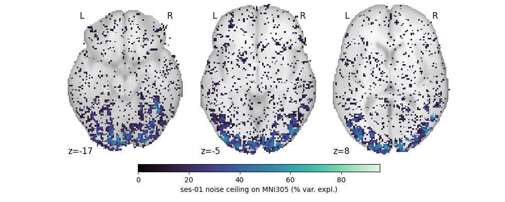
Visualize the MNI305 output

A good way to convince yourself the projection worked is to overlay the resampled map on the matching MNI305 anatomy and see whether high noise-ceiling voxels land where they should. Building that figure also makes a nice excuse to walk through how laion_fmri plays with the wider neuroimaging ecosystem, so the code below is intentionally a little more verbose than strictly necessary. The plan is to (i) pull the MNI305 T1w and brain mask from templateflow, (ii) use nilearn to multiply the T1w by the brain mask and crop to the brain’s bounding box so the backdrop shows cortex rather than skull and air, (iii) threshold the noise-ceiling map at 10% variance explained, and (iv) overlay the result on the prepared anatomy. This is the typical pattern for any group-level figure on this dataset.

import matplotlib.pyplot as plt
import seaborn as sns
from matplotlib.colors import Normalize
from nilearn import plotting
from nilearn.image import crop_img, math_img
from templateflow.api import get as tflow_get

# use templateflow to get the mni305 template
mni305_t1w = tflow_get(
    "MNI305", suffix="T1w", extension=".nii.gz",
)
mni305_brain_mask = tflow_get(
    "MNI305", suffix="mask", desc="brain", extension=".nii.gz",
)

# Templateflow ships a head T1w and a brain mask for MNI305 but
# no brain-extracted T1w directly. Thus, the T1w is multiplied
# by the brain mask to drop the skull / dura / air and then
# cropped to the brain's bounding box so plot_stat_map renders
# only the cortex.
mni305_bg = crop_img(
    math_img(
        "img * mask",
        img=str(mni305_t1w), mask=str(mni305_brain_mask),
    )
)

# define the colormap and data range
mako_cmap = sns.color_palette("mako", as_cmap=True)
nc_vmax = float(nc.max())

# define the NC threshold and cuts to plot. The threshold is
# shared with the surface figure further down so colors read
# the same way on both.
threshold = 10.0
cuts = [-17, -5, 8]

# set up the figure
fig = plt.figure(figsize=(10, 4), facecolor="white")
gs = fig.add_gridspec(2, 1, height_ratios=[1, 0.05], hspace=0.1)
fig.subplots_adjust(top=0.98, bottom=0.15)
strip_gs = gs[0].subgridspec(1, 3, wspace=0.05)
axes = [fig.add_subplot(strip_gs[0, i]) for i in range(3)]

# set up the colorbar strip, narrowed to match the surface
# figure's colorbar width-vs-figure-width proportion
cbar_strip_gs = gs[1].subgridspec(
    1, 3, width_ratios=[0.15, 0.7, 0.15],
)
cbar_ax = fig.add_subplot(cbar_strip_gs[0, 1])

# plot the different cuts
for ax, z in zip(axes, cuts):
    ax.set_facecolor("white")
    plotting.plot_stat_map(
        mni305_img, bg_img=mni305_bg, axes=ax,
        display_mode="z", cut_coords=[z],
        cmap=mako_cmap, vmax=nc_vmax, colorbar=False,
        black_bg=False, threshold=threshold,
    )

# define and render the colorbar
sm = plt.cm.ScalarMappable(
    cmap=mako_cmap, norm=Normalize(vmin=0, vmax=nc_vmax),
)
fig.colorbar(
    sm, cax=cbar_ax, orientation="horizontal",
    label=f"{session} noise ceiling on MNI305 (% var. expl.)",
)
plt.show()

Surface route: T1w → fsaverage (single hemisphere)

Surface projections take a two-step trip: vol_to_surf lifts the volume onto the subject’s fsnative mesh, then a surface resampler carries it across to fsaverage. The hemisphere can be picked with hemi="L" or "R" and the mesh density with fsaverage_density. The default fsaverage5 (10k vertices per hemi) is fast; fsaverage6 (41k) and fsaverage (164k) trade compute time for finer detail.

nc_fsavg_lh = sub.to_template(nc, "fsaverage", hemi="L")
nc_fsavg_rh = sub.to_template(nc, "fsaverage", hemi="R")
print(f"fsaverage5 L: {nc_fsavg_lh.shape}")
print(f"fsaverage5 R: {nc_fsavg_rh.shape}")

# Higher density (fsaverage6 / 41k vertices per hemi)
nc_fsavg6_lh = sub.to_template(
    nc, "fsaverage", hemi="L", fsaverage_density="fsaverage6",
)
print(f"fsaverage6 L: {nc_fsavg6_lh.shape}")

fsaverage5 L: (10242,)
fsaverage5 R: (10242,)
fsaverage6 L: (40962,)

Re-project the noise ceiling at the full fsaverage density

To showcase the high resolution in the visualization, the projection is re-run to fsaverage (164k vertices per hemi). However, the choice of the surface depends on the intended use case and analyses.

nc_fsavg_lh_hi = sub.to_template(
    nc, "fsaverage", hemi="L", fsaverage_density="fsaverage",
)
nc_fsavg_rh_hi = sub.to_template(
    nc, "fsaverage", hemi="R", fsaverage_density="fsaverage",
)
print(f"fsaverage L (164k): {nc_fsavg_lh_hi.shape}")
print(f"fsaverage R (164k): {nc_fsavg_rh_hi.shape}")

fsaverage L (164k): (163842,)
fsaverage R (164k): (163842,)

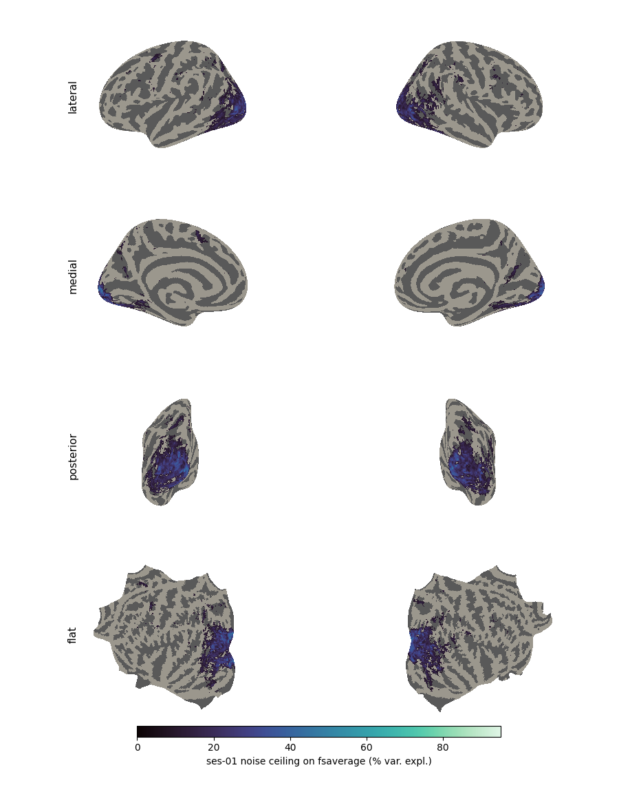
Configure the gyri / sulci backdrop and the view layout

Two things make a surface figure read well: a clear anatomical backdrop (so the reader can tell where on the cortex they are looking) and a layout that shows enough viewpoints to cover the regions of interest. The cell below sets up both at once. The backdrop encodes gyri / sulci in two shades of gray so the noise-ceiling overlay stays the most colorful element on the plot, and the view layout is a per-row tuple that pairs each anatomical view (lateral, medial, posterior, flat) with the matching fsaverage mesh. This is the same recipe to reach for whenever a surface figure has to be compared cleanly against a volume one further down.

from matplotlib.colors import ListedColormap, to_rgba
from nilearn import datasets, surface

# define colors for the surface plots
GYRI_HEX = "#9B978D"
SULCI_HEX = "#595959"
N_NC_BINS = 64
fsavg = datasets.fetch_surf_fsaverage("fsaverage")  # 164k

# stack the gyri / sulci greys ahead of 64 mako bins so a single
# integer label per vertex covers both anatomy and data
mako_bins = [
    mako_cmap(i / (N_NC_BINS - 1)) for i in range(N_NC_BINS)
]
composite_cmap = ListedColormap(
    [(1, 1, 1, 1), to_rgba(GYRI_HEX), to_rgba(SULCI_HEX)]
    + mako_bins
)

# define a per-row layout with multiple views:
# (label, (lh_view, rh_view), lh_mesh, rh_mesh).
view_rows = [
    ("lateral",
     ("lateral", "lateral"),
     fsavg.infl_left, fsavg.infl_right),
    ("medial",
     ("medial", "medial"),
     fsavg.infl_left, fsavg.infl_right),
    ("posterior",
     ("posterior", "posterior"),
     fsavg.infl_left, fsavg.infl_right),
    ("flat",
     ((90, -90), (90, -90)),
     fsavg.flat_left, fsavg.flat_right),
]

# define a shared spatial extent for both flat panels.
# Without this, matplotlib 3D auto-fits each panel to its own
# mesh and the two end up at slightly different vertical
# positions
lh_flat_verts = surface.load_surf_mesh(fsavg.flat_left)[0]
rh_flat_verts = surface.load_surf_mesh(fsavg.flat_right)[0]
flat_all = np.concatenate([lh_flat_verts, rh_flat_verts])
flat_xlim = (flat_all[:, 0].min(), flat_all[:, 0].max())
flat_ylim = (flat_all[:, 1].min(), flat_all[:, 1].max())
flat_zlim = (flat_all[:, 2].min(), flat_all[:, 2].max())

[fetch_surf_fsaverage] Dataset found in $HOME/nilearn_data/fsaverage

Render the multi-view surface grid

With the layout and the composite colormap in place, the goal of this cell is to render four anatomical views per hemisphere (lateral, medial, posterior, flat) using the same noise- ceiling threshold and color range as the volume figure above. Keeping both figures on the same scale matters because it lets the reader make a direct visual comparison: a noise-ceiling value of, say, 0.4 produces the exact same color whether it is shown on the MNI305 slices or on the inflated fsaverage surface, and the thresholded boundary marks the same cut on both sides. Without that alignment, two figures of the same underlying data can look misleadingly different.

# setup the figure
fig = plt.figure(figsize=(9.0, 11.5), facecolor="white")
gs = fig.add_gridspec(
    5, 1, height_ratios=[1, 1, 1, 1, 0.06], hspace=0.02,
)
fig.subplots_adjust(top=0.99, bottom=0.07, left=0.04, right=0.99)

# loop over views
for row_idx, (label, views, mesh_l, mesh_r) in enumerate(view_rows):
    row_gs = gs[row_idx].subgridspec(1, 2, wspace=0.02)
    for col_idx, (mesh, arr, curv_path, hemi_full, view) in (
        enumerate(zip(
            (mesh_l, mesh_r),
            (nc_fsavg_lh_hi, nc_fsavg_rh_hi),
            (fsavg.curv_left, fsavg.curv_right),
            ("left", "right"),
            views,
        ))
    ):
        ax = fig.add_subplot(row_gs[0, col_idx], projection="3d")
        curv = surface.load_surf_data(curv_path)
        roi_map = np.where(curv < 0, 1.0, 2.0)
        above = arr >= threshold
        if above.any():
            norm = np.clip(arr / nc_vmax, 0.0, 1.0)
            bin_idx = (norm * (N_NC_BINS - 1)).astype(np.int32)
            roi_map[above] = 3.0 + bin_idx[above]
        plotting.plot_surf_roi(
            mesh, roi_map=roi_map,
            hemi=hemi_full, view=view,
            cmap=composite_cmap, vmin=0, vmax=2 + N_NC_BINS,
            colorbar=False, figure=fig, axes=ax,
        )
        ax.set_anchor("C")
        if label == "flat":
            ax.set_xlim(flat_xlim)
            ax.set_ylim(flat_ylim)
            ax.set_zlim(flat_zlim)
        if col_idx == 0:
            ax.text2D(
                -0.05, 0.5, label,
                transform=ax.transAxes,
                rotation=90, ha="center", va="center",
                fontsize=11,
            )

# define and render the colorbar
cbar_strip_gs = gs[4].subgridspec(
    1, 3, width_ratios=[0.15, 0.7, 0.15],
)
cbar_ax = fig.add_subplot(cbar_strip_gs[0, 1])
sm_surf = plt.cm.ScalarMappable(
    cmap=mako_cmap,
    norm=Normalize(vmin=0, vmax=nc_vmax),
)
fig.colorbar(
    sm_surf, cax=cbar_ax, orientation="horizontal",
    label=f"{session} noise ceiling on fsaverage (% var. expl.)",
)
plt.show()

Both hemispheres at once (hemi=None)

If both hemispheres should be returned in a single call, hemi can be left at its default of None. The return value becomes a dict keyed by "L" and "R", with each value the same 1-D array shape as the single-hemi call above.

# project both hemispheres at once
both_hemis = sub.to_template(nc, "fsaverage")
print(f"Returned: {type(both_hemis).__name__} with keys "
      f"{sorted(both_hemis)}")
print(f"L shape: {both_hemis['L'].shape}")
print(f"R shape: {both_hemis['R'].shape}")

Returned: dict with keys ['L', 'R']
L shape: (10242,)
R shape: (10242,)

Batched input: (n_trials, n_voxels) → (n_trials, n_vertices)

Single-trial analyses usually start from a (n_trials, n_voxels) array rather than a single summary map. The same to_template call accepts the 2-D input and keeps the trial axis on the output: a 4-D NIfTI for volume targets, a 2-D (n_trials, n_vertices) array for surface targets. Inputs are sized to the brain mask. For ROI-masked betas, scatter them back into the brain-mask shape first with Subject.to_nifti().

# load the first eight single-trial betas at the brain-mask
# resolution. ``streaming=True`` keeps peak memory low while
# the session NIfTI is decompressed and read volume by volume.
betas = sub.get_betas(session=session, streaming=True)
batch_full = betas[:2]
print(f"Input batch:  {batch_full.shape}")

# project the batched input onto MNI305 (4-D NIfTI, trial axis
# trailing)
mni305_batch = sub.to_template(batch_full, "MNI305")
print(f"MNI305 4-D:   shape={mni305_batch.shape}")

# project the batched input onto fsaverage5 (2-D, trial axis
# leading)
fsavg_batch = sub.to_template(batch_full, "fsaverage", hemi="L")
print(f"fsavg5 batch: {fsavg_batch.shape}")

Input batch:  (2, 272080)
MNI305 4-D:   shape=(172, 220, 156, 2)
fsavg5 batch: (2, 10242)

Surface → surface (fsnative → fsaverage)

If the data already lives on the subject’s fsnative mesh (e.g., a surface-based ROI mask, surface-fit betas, or anything else in surface space), surface_to_template skips the volume step and resamples straight onto fsaverage. Pass a per-hemi array with hemi="L" or "R", or a {"L": ..., "R": ...} dict for both hemispheres in one call. The input vertex count has to match the subject’s fsnative mesh.

# pull an fsnative-space ROI mask from disk
roi_data = sub.get_roi_data(roi, format="func.gii", hemi="L")
fsnative_lh = roi_data[roi]["gii"]["hemi-L"]["func.gii"]
print(f"fsnative L mesh size: {fsnative_lh.shape}")

# resample the fsnative ROI mask onto fsaverage5
ffa1_on_fsavg = sub.surface_to_template(
    fsnative_lh.astype(np.float32), hemi="L",
)
print(f"FFA1 on fsavg5 L:     {ffa1_on_fsavg.shape}")
print(f"Vertices marked ROI:  {int((ffa1_on_fsavg > 0.5).sum())}")

fsnative L mesh size: (148371,)
FFA1 on fsavg5 L:     (10242,)
Vertices marked ROI:  12

Direction-specific entry points

to_template infers the route from the target name. If the input / output direction should be visible at the call site, three direction-specific methods do the same work under more descriptive names:

• volume_to_template(values, target): volume in, volume out (e.g. T1w → MNI305).

• volume_to_surface(values, target="fsaverage"): volume in, surface out (e.g. T1w → fsaverage).

• surface_to_template(values, target="fsaverage", hemi=...): surface in, surface out (e.g. fsnative → fsaverage).

A target that doesn’t match the chosen direction raises ValueError at the call site, so a wrong combination is caught before any data moves.

# direct volume-to-volume projection
vol_mni = sub.volume_to_template(nc, "MNI305")
# direct volume-to-surface projection
vol_surf_l = sub.volume_to_surface(nc, hemi="L")
print(f"volume_to_template(MNI305):   {vol_mni.shape}")
print(f"volume_to_surface(L):         {vol_surf_l.shape}")

# For example, when the target doesn't match the chosen
# direction (uncomment locally to see the raised ValueError;
# kept commented so the gallery build does not crash):
# sub.volume_to_template(nc, "fsaverage")  # ValueError

volume_to_template(MNI305):   (172, 220, 156)
volume_to_surface(L):         (10242,)