GLMsingle Beta Estimates

Single-trial betas are voxelwise estimates of the BOLD response to each individual stimulus presentation. They are a compact summary of the stimulus-driven activity in the dataset and the usual starting point for encoding models, decoding, and representational similarity analyses (RSA). If you want to relate brain activity to a specific image, you are at the right place to start.

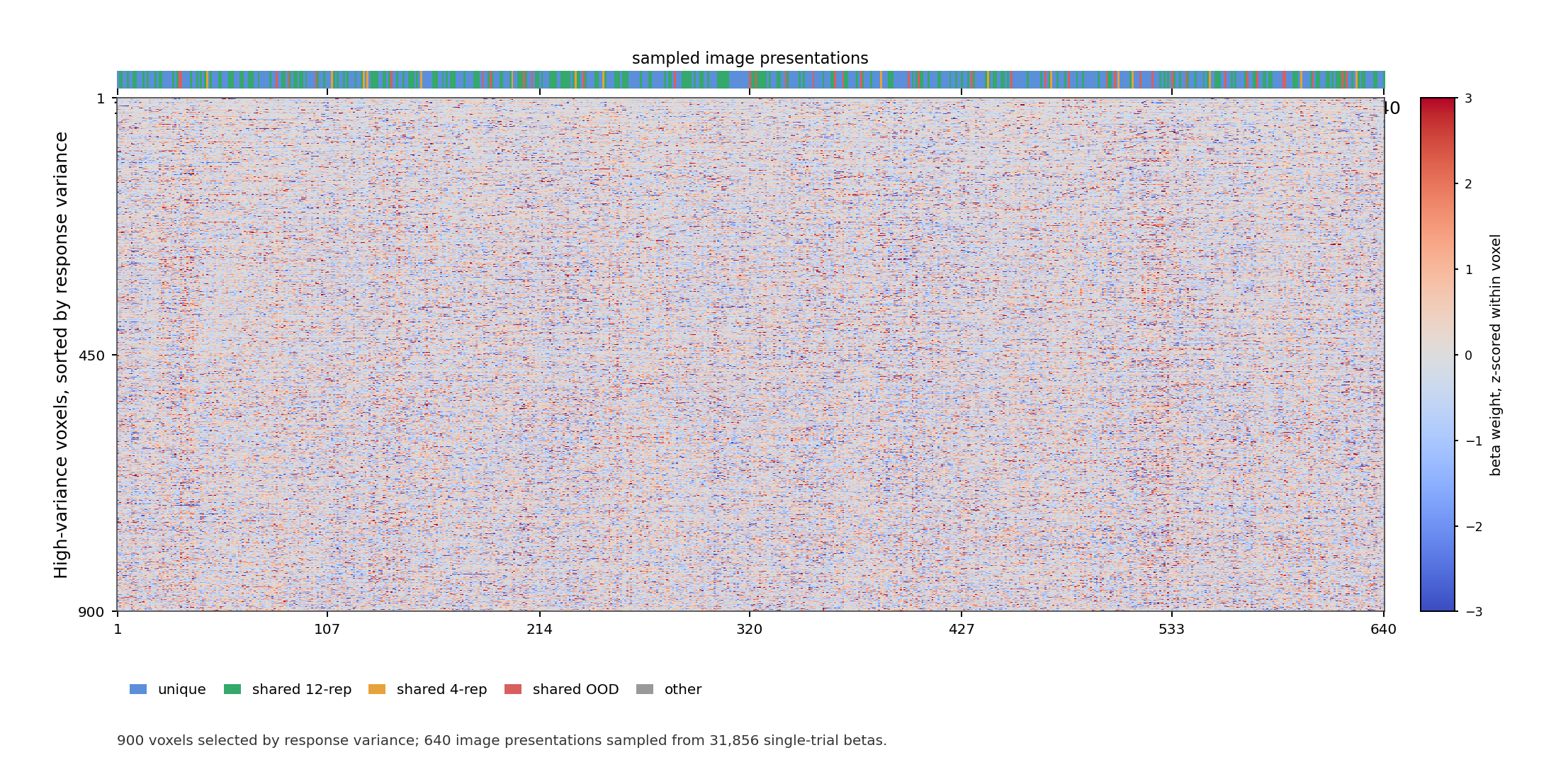
GLMsingle TYPED beta carpet plot for sub-03. Columns are sampled image presentations, rows are high-variance voxels sorted by response variance, and colors show beta weights z-scored within each voxel.

Overview

GLMsingle (Prince et al., 2022) is a toolbox for estimating single-trial BOLD response amplitudes from event-related fMRI. It returns one beta per trial per voxel and improves on a standard GLM in three ways: it picks the best-fitting hemodynamic response function (HRF) for each voxel from a library of 20 HRFs, it derives data-driven nuisance regressors via GLMdenoise to remove structured noise (motion artefacts, physiological artefacts, scanner drift), and it stabilises trial estimates with fractional ridge regression. These steps make betas more reliable, especially in rapid event-related designs where trial responses overlap. The toolbox is available at https://github.com/cvnlab/GLMsingle.

Method	GLMsingle (Prince et al., 2022) on tedana optimally-combined BOLD
GLMsingle version	Python, v1.2 (cvnlab/GLMsingle)
Input data	tedana optimally-combined BOLD from a 3-echo acquisition (the three echoes are combined into a single weighted timeseries before fitting); see Preprocessing
Output shape	(143, 143, 143, n_trials) per session; n_trials varies per session (typically 1044 or 1066)
Available spaces	T1w native (volumetric), 1.778 mm isotropic
Beta versions provided	TYPED (b4) only (FITHRF_GLMDENOISE_RR — full GLMsingle pipeline with HRF fitting, GLMdenoise, and fractional ridge)
Noise ceilings	per-voxel, both per-session and cross-session maps (see Noise Ceilings)

File Organization

Each subject folder has one subfolder per session, all sessions following the same layout. Example for sub-01/ses-01:

sub-01/
└── ses-01/
    └── func/
        ├── sub-01_ses-01_task-images_desc-GLMsingle_summary.json                                # session-level run summary
        ├── sub-01_ses-01_task-images_desc-SingletrialBetas_trials.tsv                           # trial-to-stimulus mapping
        ├── sub-01_ses-01_task-images_desc-SingletrialBetas_trials.json
        ├── sub-01_ses-01_task-images_space-T1w_desc-GLMsingle_model.h5                          # full GLMsingle output (b4, R², ...)
        ├── sub-01_ses-01_task-images_space-T1w_desc-GLMsingle_model.json
        ├── sub-01_ses-01_task-images_space-T1w_stat-effect_desc-SingletrialBetas_statmap.nii.gz # 4D single-trial betas
        ├── sub-01_ses-01_task-images_space-T1w_stat-effect_desc-SingletrialBetas_statmap.json
        ├── sub-01_ses-01_task-images_space-T1w_stat-rsquare_desc-R2_statmap.nii.gz              # variance explained per voxel
        ├── sub-01_ses-01_task-images_space-T1w_stat-rsquare_desc-R2_statmap.json
        ├── sub-01_ses-01_task-images_space-T1w_desc-Noiseceiling_statmap.nii.gz                 # within-session noise ceiling
        ├── sub-01_ses-01_task-images_space-T1w_desc-Noiseceiling_statmap.json
        ├── sub-01_ses-01_task-images_space-T1w_desc-HRFindex_dseg.nii.gz                        # selected HRF (0-19) per voxel
        ├── sub-01_ses-01_task-images_space-T1w_desc-HRFindex_dseg.json
        ├── sub-01_ses-01_task-images_space-T1w_desc-Fracridge_statmap.nii.gz                    # ridge fraction per voxel
        ├── sub-01_ses-01_task-images_space-T1w_desc-Fracridge_statmap.json
        └── figures/                                                                             # diagnostic plots
...

sub-01_task-images_desc-GLMsingle_summary.json                                                   # subject-level aggregation summary
sub-01_task-images_space-T1w_desc-Noiseceiling4rep_statmap.nii.gz                                # across-session noise ceiling (4-rep stimuli)
sub-01_task-images_space-T1w_desc-Noiseceiling4rep_statmap.json
sub-01_task-images_space-T1w_desc-Noiseceiling12rep_statmap.nii.gz                               # across-session noise ceiling (12-rep stimuli)
sub-01_task-images_space-T1w_desc-Noiseceiling12rep_statmap.json
sub-01_task-images_space-T1w_desc-NoiseceilingAllrep_statmap.nii.gz                              # across-session noise ceiling (all repeats)
sub-01_task-images_space-T1w_desc-NoiseceilingAllrep_statmap.json
sub-01_task-images_space-T1w_stat-rsquare_desc-R2mean_statmap.nii.gz                             # mean R² across sessions
sub-01_task-images_space-T1w_stat-rsquare_desc-R2mean_statmap.json

The 4D NIfTI holds the betas as one volume per trial. The HDF5 model holds the same betas plus (intermediate) diagnostic outputs (noise pool, PC regressors, cross-validation metrics; useful for inspection but not needed for typical use). JSON sidecars record acquisition and processing parameters. The figures/ folder contains diagnostic images (R², noise ceiling, HRF index mosaic, etc.).

A few notes: blank trials (fixation-only without image) are dropped before fitting and do not appear in the betas or in trials.tsv. Only runs 01-12 are used per session, any extra runs are skipped. Runs with too few timepoints (specifically relating to session 31) are excluded and logged in the session summary JSON. So far there is no quality flag included in trials.tsv (indicating if the subject blinked, moved, etc.); we may add it later.

Beta Versions

GLMsingle internally fits four progressively more fine-tuned models, labelled TYPEA, TYPEB, TYPEC, and TYPED. Each stage adds one of the toolbox’s core improvements. Only the final stage TYPED is shipped with this dataset. The earlier stages are intermediate steps in the algorithm but we describe them here briefly so the origin of the final betas is clear.

Version	Name	Description
TYPEA	ASSUMEHRF	Rough on-off (any stimulus vs no stimulus) general linear model with a fixed canonical HRF. Used internally to identify voxels with no task response at all (the noise pool). Its betas are not saved.
TYPEB	FITHRF	Single-trial GLM that picks the best fitting HRF per voxel from the 20-HRF library. The betas are again not saved, only the HRF index per voxel is shipped.
TYPEC	FITHRF_GLMDENOISE	TYPEB plus GLMdenoise nuisance regressors derived from the noise pool, with the number of regressors chosen via cross-validation. Betas are not saved.
TYPED	FITHRF_GLMDENOISE_RR	TYPEC plus fractional ridge regression (RR), with a regularisation strength for each voxel chosen by cross-validation. These are the betas that are actually shipped.

A few challenges to keep in mind when using the TYPED betas. Ridge regression shrinks beta magnitudes toward zero, so betas are reliable in a relative sense (good for encoding, decoding, RSA, and contrasts) but should not be read as raw percent signal change. Voxels are regularised with different strength, so absolute magnitudes are not strictly comparable across voxels. For analyses like ROI averages or group maps it is safer to z-score within a session before averaging. A small fraction of voxels near the brain mask edge or in dropout regions may contain NaN; check for them (or check the sidecar JSON).

Noise Ceilings

From the single-trial betas produced by GLMsingle, we derived noise ceiling (NC) estimates that quantify the fraction of variance at each voxel that is driven by the stimulus rather than noise. Two complementary maps are provided: both are computed by us on top of GLMsingle’s single-trial betas, with the per-session NC using repeats within a single session and the cross-session NC averaging repeats across all sessions of a participant.

The per-session and cross-session noise ceilings are volumetric statmaps, yielding one value per voxel within the brain mask (anything outside the brain is 0). No ROI-level aggregation is built in; any ROI needs to be mapped first (e.g. for visual vs. non-visual medians).

Both maps are produced by the same function, implementing NSD’s ncsnr formula (Allen et al., 2022). Betas are z-scored per voxel (per run for the single-session case, per session for the cross-session case) so that total variance is ~1, and repeated presentations of the same image are used to estimate noise variance as the mean within-image residual variance. The signal variance follows as \(\sigma^2_{\text{signal}} = \max(0,\, 1 - \sigma^2_{\text{noise}})\), where \(\sigma^2\) denotes variance (and \(\sigma\) the standard deviation). The noise-ceiling SNR is \(\text{ncsnr} = \sigma_{\text{signal}} / \sigma_{\text{noise}}\), converted to a percentage via

\[\mathrm{NC} = 100 \times \frac{\text{ncsnr}^2}{\text{ncsnr}^2 + \overline{1/n_c}}\]

where \(n_c\) is the number of repeats of image \(c\), and the mean across images corrects for unequal repetition counts. The two maps differ only in their input: the per-session NC uses repeats within one session, while the cross-session NC averages repeats across all sessions, thereby yielding more stable, higher values.

These values lie between 0 and 100 and can be read as the best \(R^2\) (the fraction of variance a model explains) an encoding model could possibly achieve at that voxel. An NC of 40, for example, means that even a perfect stimulus-based model could explain at most 40 % of the variance in the betas and the remaining 60 % is trial-to-trial noise that no stimulus-based model can capture. Thus, NC is a strict upper bound on encoding-model performance, not a claim about how much “true signal” is physically present in the voxel.

As this boundary directly sets the ceiling for model evaluation, an encoding model reaching \(R^2 = 30 \%\) at a voxel with \(\mathrm{NC} = 40 \%\) is in fact explaining 75 % of the explainable variance (30/40). Voxels with NC near zero are noise-dominated and should be excluded or down-weighted in downstream analyses. As we show visual stimuli in the main experiment, the high NC values concentrate primarily in visual cortex and grow with additional sessions, as reflected in the color scales of the figures below: the meaningful range extends once repeats are averaged across multiple sessions.

Todo

Add figures: sub-03_ses-01_nc (per-session NC) and sub-03_ses-all_nc (cross-session NC).

Noise ceiling map for an example subject. (placeholder — replace with actual figure)

Relation to Stimuli

Each session folder contains a trial TSV (_desc-SingletrialBetas_trials.tsv) that maps each beta volume to the stimulus shown on that trial. It has four columns: session, run, beta_index (counting from 0 in order of trial appearance within the session), and label (the stimulus image filename).

Each row in trials.tsv corresponds to a volume in the 4D beta NIfTI, or equivalently a column in the HDF5 betasmd matrix. The label column is the join key for the stimulus metadata.

Repeated presentations of the same stimulus are kept as separate trials and never averaged. A typical session contains around 1044–1066 trials covering ~770 unique stimuli, so a few hundred trials per session are repeats. Cross-session repeats are likewise stored as separate single-trial betas. Users are free to average across repeats if they want, using the label column to group trials. For information on which stimuli are reserved for testing, see Train / Test Splits.

Loading the Data

The recommended way to load betas is through the laion_fmri package, which wraps the file layout above with named accessors:

from laion_fmri.subject import load_subject

sub = load_subject("sub-01")
betas = sub.get_betas(session="ses-01")          # (n_trials, n_voxels)
trials = sub.get_trial_info(session="ses-01")    # pandas DataFrame; `label` column joins to stimuli

See Load for the full API: ROI filters, noise ceiling thresholding, multi-session access, brain-space mapping, and the PyTorch dataset wrapper.