Loading Data

This example walks through the loaders that turn a downloaded subject directory into usable arrays: single-trial betas, noise-ceiling maps, ROI masks, and stimulus images. The goal is to give a feel for what each accessor does, how its arguments interact, and which patterns to reach for in real analyses.

Every accessor maps to one file in the bucket and returns the raw contents of that file. Combining sessions, averaging across trials, or rebinning is therefore the caller’s responsibility, since the loaders deliberately do not hide that step. That makes the data easy to plug into custom pipelines but also means a naive call without an ROI filter can pull a full session of beta values into memory at once.

A second important choice surfaces early: which brain mask defines the voxel axis. Two sources are available and the same mask_source choice cascades through every voxel-axis loader.

• source="anatomical" (default): the anatomically-derived mask shipped under derivatives/anatomical/. Broader, since it includes voxels with no functional fit.

• source="rsquare": derived on the fly from the subject-level mean-R^2 map; only voxels with any non-zero GLMsingle fit are counted. Narrower, functional-only.

Note

Run plot_01 first so at least one subject is downloaded into the shared quickstart directory. A single session of full-brain betas is ~1000 trials × ~270k voxels × 4 bytes ≈ 1 GB; pass an roi= filter to keep per-call memory in the tens of MB.

Bind the quickstart’s data directory

Like the other examples, plot_04 reuses the data directory that the quickstart sets up so the data downloaded there can be reused. dataset_initialize is a no-op once the config is already on disk.

import os

from laion_fmri.config import dataset_initialize, get_data_dir

# define and initialize the data directory
data_dir = os.environ.get(
    "LAION_FMRI_EXAMPLE_DATA_DIR",
    os.path.join(os.getcwd(), "laion_fmri_quickstart"),
)
os.makedirs(data_dir, exist_ok=True)
dataset_initialize(data_dir)

Load a subject and pick a session

The entry point to per-subject data is load_subject(). It returns a Subject wrapping the on-disk files; every loader call further down is a method on that object. The example pins subject_id, session, and a primary roi so the same trio can be reused across cells.

from laion_fmri.subject import load_subject

# set subject information
subject_id = "sub-01"
session = "ses-01"
roi = "FFA1"

# load and inspect the subject
sub = load_subject(subject_id)
print(f"Subject: {subject_id} | session: {session}")
print(f"Voxels in brain mask: {sub.get_n_voxels()}")

# list the available ROIs and pick the primary one
available_rois = sub.get_available_rois()
print(f"Primary ROI: {roi}")

Subject: sub-01 | session: ses-01
Voxels in brain mask: 272080
Primary ROI: FFA1

Two brain-mask sources

Before any voxel-axis array is loaded, the brain mask that defines that axis has to be picked. The package exposes the choice as a mask_source kwarg on every voxel-axis loader (get_betas, get_noise_ceiling, to_nifti, get_voxel_coordinates); picking it once at one loader keeps the voxel axis consistent across all the others. The two options match the two masks the dataset ships:

• mask_source="anatomical" (default): the anatomically-derived brain mask shipped under derivatives/anatomical/. Usually wider, since brain voxels with no functional fit come along.

• mask_source="rsquare": voxels with any non-zero GLMsingle fit. Smaller, functional-only.

Which one to pick depends on the analysis: the anatomical mask is the right choice when comparing against the published baselines (they use it), the rsquare mask is preferable for analyses that should exclude voxels GLMsingle could not fit.

# compare voxel counts between the two mask sources
rsq_mask = sub.get_brain_mask(source="rsquare")
anat_mask = sub.get_brain_mask(source="anatomical")
print(f"rsquare-derived voxels: {rsq_mask.sum()}")
print(f"anatomical voxels:      {anat_mask.sum()}")

# Resolution: ``res="1pt8"`` (default) matches the functional
# voxel grid, so a 1-D mask of length ``X*Y*Z`` indexes the beta
# arrays voxel-for-voxel. Pass ``res=None`` for the
# full-resolution anatomical mask (same T1w coordinate space,
# finer voxel grid); useful when working with the full-res T1w
# / T2w volumes directly, but the array is larger and no
# longer indexes the per-voxel loaders below.
anat_full = sub.get_brain_mask(source="anatomical", res=None)
print(f"anatomical full-res voxels: {anat_full.sum()}")

# A mask is picked once at any voxel-axis loader and the rest
# of the pipeline follows. The loaders pin ``res="1pt8"``
# internally so the returned voxel axis is always 1-D over the
# functional voxel grid regardless of which ``mask_source`` is
# chosen.
nc_rsq = sub.get_noise_ceiling(
    session=session, mask_source="rsquare",
)
nc_anat = sub.get_noise_ceiling(
    session=session, mask_source="anatomical",
)
print(f"NC shape (rsquare):    {nc_rsq.shape}")
print(f"NC shape (anatomical): {nc_anat.shape}")

rsquare-derived voxels: 271557
anatomical voxels:      272080
anatomical full-res voxels: 2987111
NC shape (rsquare):    (271557,)
NC shape (anatomical): (272080,)

Single-trial betas for one session

Single-trial betas are the main per-stimulus signal the dataset exposes; loading them is the most common thing a Subject does. get_betas returns an (n_trials, n_voxels) array, and the voxel axis is the brain mask that was just picked.

Two filtering mechanisms keep the array small and the analysis focused. roi= picks a single ROI, a category, an ROI list, or "all" for the union of every ROI; the result is a voxel-axis subset that is one to two orders of magnitude smaller than the full mask, which matters because a full-brain session is roughly 1 GB. nc_threshold= is the noise-ceiling-based filter. It drops voxels below the given ceiling so the loader returns only the reliable voxels. The two filters compose, so combining roi= and nc_threshold= is the typical pattern for region-restricted analyses on reliable voxels only.

# load betas for a single ROI
if roi is not None:
    betas_roi = sub.get_betas(session=session, roi=roi)
    print(f"{roi} ROI:           {betas_roi.shape}")

# filter by noise ceiling
betas_nc = sub.get_betas(session=session, nc_threshold=0.2)
print(f"NC > 0.2:            {betas_nc.shape}")

# combine ROI + NC filtering
if roi is not None:
    betas_both = sub.get_betas(
        session=session, roi=roi, nc_threshold=0.3,
    )
    print(f"ROI + NC > 0.3:      {betas_both.shape}")

FFA1 ROI:           (1044, 222)
NC > 0.2:            (1044, 132612)
ROI + NC > 0.3:      (1044, 189)

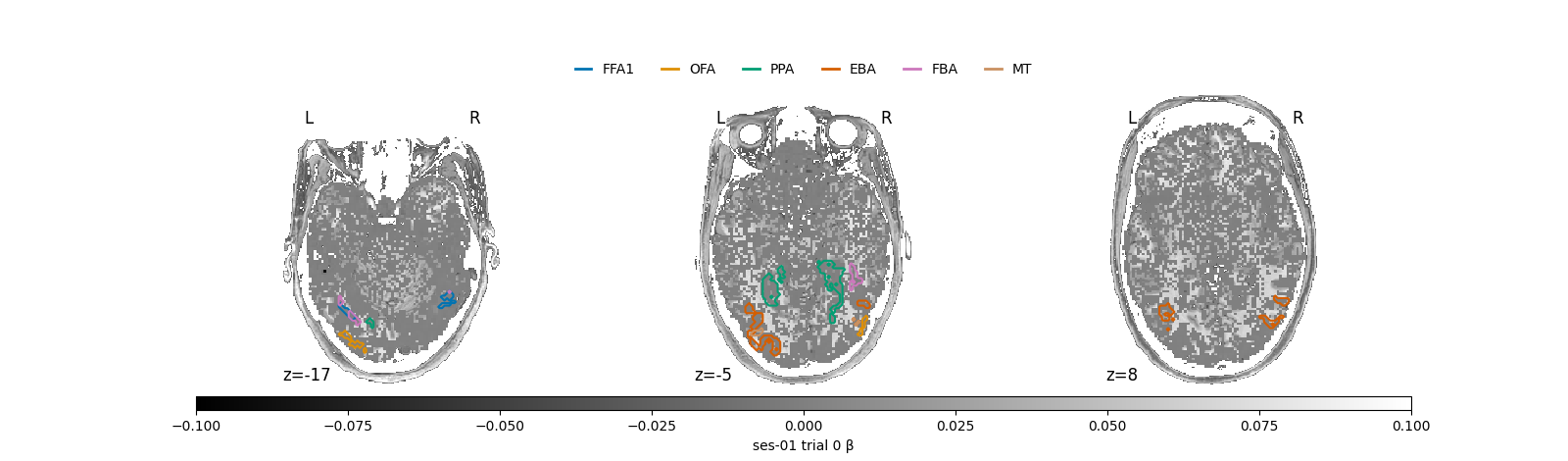
Visualize the first trial with ROI contour overlays

A picture often confirms the array shapes are real and not just numbers. Overlaying the canonical face / body / place ROI contours on a single trial’s response provides a concrete check on two things at once: that the ROIs sit where they should, and that the betas have plausible signal in roughly the right anatomical neighborhood.

Single trials are inherently noisy and stimulus-dependent, so not every ROI will show a hotspot on every trial, the expected outcome is plausible signal somewhere near the contours rather than uniform noise. The betas are rendered in grayscale so the colored ROI contours stay visually dominant.

import warnings

import numpy as np
import matplotlib.pyplot as plt
import seaborn as sns
from matplotlib.colors import ListedColormap, Normalize
from matplotlib.lines import Line2D
from nilearn import plotting

# Nilearn warns about NaN / inf voxels from GLMsingle non-fits;
# they're outside the brain mask and don't affect the rendering.
warnings.filterwarnings(
    "ignore",
    message="Non-finite values detected",
    category=UserWarning,
)

# pick a scratch directory under the shared data dir for the
# derivative NIfTIs this example writes; the path is
# auto-sanitized in the rendered gallery
import pathlib

scratch_dir = pathlib.Path(data_dir) / "tmp"
scratch_dir.mkdir(exist_ok=True)

# define the anatomical backdrop and a grayscale beta colormap
# so the colored ROI contours stay visually dominant
bg_img = str(sub.get_t1w())
stat_cmap = "gray"
overlay_rois = ("FFA1", "OFA", "PPA", "EBA", "FBA", "MT")
roi_colors = dict(
    zip(overlay_rois, sns.color_palette("colorblind")),
)

# scatter the first trial's betas back to NIfTI for plotting
first_beta = sub.get_betas(session=session, streaming=True)[0]
beta_path = str(
    scratch_dir / f"{subject_id}_{session}_trial0_full.nii.gz"
)
sub.to_nifti(first_beta, beta_path)

# scatter each ROI mask to NIfTI for the contour overlays
roi_paths = {}
for r in overlay_rois:
    p = str(scratch_dir / f"{subject_id}_roi_{r}.nii.gz")
    sub.to_nifti(sub.get_roi_mask(r).astype("float32"), p)
    roi_paths[r] = p

# pick a symmetric vmax and the axial cuts to plot
vmax = float(np.percentile(np.abs(first_beta), 99))
cuts = [-17, -5, 8]

# set up the figure with three slots: top legend strip, the
# three panels, bottom colorbar
fig = plt.figure(figsize=(16, 4.7))
gs = fig.add_gridspec(
    3, 1, height_ratios=[0.10, 1, 0.05], hspace=0.1,
)
legend_ax = fig.add_subplot(gs[0])
legend_ax.axis("off")
strip_gs = gs[1].subgridspec(1, 3, wspace=0.05)
axes = [fig.add_subplot(strip_gs[0, i]) for i in range(3)]
cbar_ax = fig.add_subplot(gs[2])

# plot one cut per panel and overlay every ROI contour
for ax, z in zip(axes, cuts):
    display = plotting.plot_stat_map(
        beta_path, bg_img=bg_img, axes=ax,
        display_mode="z", cut_coords=[z],
        cmap=stat_cmap, vmax=vmax, colorbar=False,
        black_bg=False, threshold=0.5,
    )
    for roi, color in roi_colors.items():
        display.add_contours(
            roi_paths[roi], levels=[0.5],
            colors=[color], linewidths=1.5,
        )

# build a color/legend strip across the top so every contour is
# named
proxies = [
    Line2D([0], [0], color=c, lw=2.0, label=r)
    for r, c in roi_colors.items()
]
legend_ax.legend(
    handles=proxies, loc="center", ncol=len(overlay_rois),
    frameon=False, handlelength=1.2,
)

# define and render the colorbar
sm = plt.cm.ScalarMappable(
    cmap=stat_cmap, norm=Normalize(vmin=-vmax, vmax=vmax),
)
fig.colorbar(
    sm, cax=cbar_ax, orientation="horizontal",
    label=f"{session} trial 0 β",
)
plt.show()

Single-trial filtering by stimulus type

Many analyses care about a specific subset of stimuli rather than every trial, for instance only the shared stimulus set when comparing across subjects, or only the subject’s unique trials for richer per-subject modeling. The stimuli= argument provides that cut directly on the loader, so the returned betas already match the desired subset.

The filter relies on the dataset-level stimulus metadata that joins trial information to stimulus IDs. When the metadata has not been uploaded to the bucket yet, the cell prints a note and skips the call rather than failing.

# filter to shared-stimulus trials when stimulus metadata is
# available
if roi is not None and sub.has_stimuli():
    betas_shared = sub.get_betas(
        session=session, roi=roi, stimuli="shared",
    )
    print(f"Shared trials:       {betas_shared.shape}")
else:
    print(
        "Skipped: stimulus subset filter needs stimuli/stimuli.tsv."
    )

Shared trials:       (469, 183)

Custom voxel mask

Sometimes the desired voxel selection is more specific than anything roi= or nc_threshold= covers on their own, for instance voxels that are inside an ROI and above a reliability threshold, or any other boolean combination of the masks the loaders expose. For those cases the mask= kwarg accepts a precomputed 1-D boolean array and uses it verbatim as the voxel selector, side-stepping the built-in filters entirely. The cell below shows the typical pattern: build the mask in Python, then hand it to get_betas.

# build a custom mask (ROI ∩ NC > 0.25) and load matching betas
if roi is not None:
    roi_mask = sub.get_roi_mask(roi)
    nc = sub.get_noise_ceiling(session=session)
    custom_mask = roi_mask & (nc > 0.25)
    print(f"Custom mask voxels: {custom_mask.sum()}")

    betas_custom = sub.get_betas(session=session, mask=custom_mask)
    print(f"Custom betas:       {betas_custom.shape}")

Custom mask voxels: 152
Custom betas:       (1044, 152)

ROI masks (multi-level query)

A lot of ROI work does not need the actual ROI data (the .gii / .label files), only the boolean voxel mask that selects the ROI’s voxels from the brain-mask axis. get_roi_mask returns exactly that, and it accepts the same multi-level grammar as roi= on get_betas: a specific ROI name, a category, "all", or a list of any of the above. Lists are de-duplicated, so overlapping voxels appear only once in the resulting mask.

# inspect the voxel counts for a single ROI, a category, and
# the full union
if available_rois:
    if roi is not None:
        single = sub.get_roi_mask(roi)
        print(f"  {roi}: {single.sum()} voxels")
    categories = sub.get_available_categories()
    if categories:
        first_cat = categories[0]
        cat_mask = sub.get_roi_mask(first_cat)
        print(f"  {first_cat} (category): {cat_mask.sum()} voxels")
    union = sub.get_roi_mask("all")
    print(f"  all: {union.sum()} voxels")

MT: 183 voxels
body (category): 1539 voxels
all: 16569 voxels

Visualize every face-category ROI

Looking at a single ROI in isolation is fine for a sanity check, but plotting an entire category in one row makes a different class of issue visible: which ROIs are present for this subject (some are absent for some subjects), how the various face areas spatially relate to each other, and whether any region looks unexpectedly small or empty, a sign that the localizer underperformed there and that the ROI is not reliable to analyze with. Doing this once, up front, surfaces problems that would otherwise turn up much later in a downstream model.

import nibabel as nib
from nilearn.plotting import find_xyz_cut_coords

# list the face-category ROIs available for this subject
face_rois = sub.get_available_rois(category="face")
if not face_rois:
    print("No face-category ROIs on disk for this subject.")
else:
    # pair each ROI with a colorblind-safe contour color
    palette = sns.color_palette("colorblind")
    n = len(face_rois)

    # set up one panel per ROI
    fig, axes = plt.subplots(1, n, figsize=(5.3 * n, 3.7))
    axes = [axes] if n == 1 else list(axes)

    # loop over ROIs and draw each contour on its own anatomical cut
    for ax, roi, color in zip(axes, face_rois, palette):
        # scatter the ROI mask to NIfTI so nilearn can read it
        roi_path = str(scratch_dir / f"{subject_id}_roi_{roi}.nii.gz")
        sub.to_nifti(
            sub.get_roi_mask(roi).astype("float32"), roi_path,
        )
        # pick the axial slice centered on the ROI's bounding box
        _, _, z = find_xyz_cut_coords(nib.load(roi_path))
        # plot the anatomical backdrop, then overlay the ROI contour
        display = plotting.plot_anat(
            bg_img, axes=ax,
            display_mode="z", cut_coords=[z],
            black_bg=False, threshold=0.1, colorbar=False,
        )
        display.add_contours(
            roi_path, levels=[0.5],
            colors=[color], linewidths=1.5,
        )
        ax.set_title(roi)
    plt.show()

Surface ROI files (.func.gii)

Some analyses live more naturally on the cortical surface than in the volume, for instance anything that relies on vertex neighborhoods or on flat-map projections. For those cases the dataset ships every ROI in three formats: the volumetric .nii.gz, a per-hemisphere .func.gii surface mask in fsnative space, and a FreeSurfer .label file. Subject.get_roi_data is the multi-format accessor that reads them straight from disk, without resampling from the volume.

The cell below pulls only the surface variant per hemisphere; the same call with a different format= would return the volume mask or the FreeSurfer label instead.

import nibabel as nib_

from laion_fmri._paths import freesurfer_surf_path
from nilearn.plotting import plot_surf_roi
from nilearn.surface import InMemoryMesh, PolyMesh, SurfaceImage

# load the per-hemisphere fsnative surface masks for one ROI
surf_roi = "FFA1"
roi_gii = sub.get_roi_data(surf_roi, format="func.gii")[surf_roi]
lh_mask = roi_gii["gii"]["hemi-L"]["func.gii"]
rh_mask = roi_gii["gii"]["hemi-R"]["func.gii"]
print(
    f"{surf_roi}: L={lh_mask.sum()} / {lh_mask.size} vertices, "
    f"R={rh_mask.sum()} / {rh_mask.size}"
)


# small helpers to read the FreeSurfer pial mesh and sulcal-depth
# map for one hemisphere from the subject's recon
def _read_pial(hemi):
    path = freesurfer_surf_path(
        get_data_dir(), subject_id, hemi, "pial",
    )
    coords, faces = nib_.freesurfer.read_geometry(str(path))
    return InMemoryMesh(coordinates=coords, faces=faces)


def _read_sulc(hemi):
    return nib_.freesurfer.read_morph_data(
        str(
            freesurfer_surf_path(
                get_data_dir(), subject_id, hemi, "sulc",
            ),
        ),
    )


# combine both hemispheres into a single PolyMesh so nilearn can
# render them side-by-side in one ventral view
pial = PolyMesh(left=_read_pial("L"), right=_read_pial("R"))
sulc = SurfaceImage(
    mesh=pial, data={"left": _read_sulc("L"), "right": _read_sulc("R")},
)

# wrap the ROI mask as a SurfaceImage; non-ROI vertices are NaN
# so only ROI vertices get colored and the rest of the surface
# keeps the gray sulcal-depth shading from ``bg_map``
roi_img = SurfaceImage(
    mesh=pial,
    data={
        "left": np.where(lh_mask, 1.0, np.nan),
        "right": np.where(rh_mask, 1.0, np.nan),
    },
)

# define a single-color teal overlay for the ROI vertices
teal_cmap = ListedColormap(["#1f9d8d"])

# set up the figure and render the ventral view
fig = plt.figure(figsize=(9, 5))
ax = fig.add_subplot(111, projection="3d")
plot_surf_roi(
    surf_mesh=pial, roi_map=roi_img,
    bg_map=sulc, hemi="both", view="ventral",
    axes=ax, colorbar=False,
    cmap=teal_cmap, bg_on_data=True,
)
ax.set_title(f"{surf_roi} (ventral view, both hemispheres)")
plt.show()

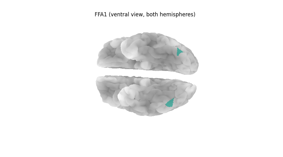
FFA1: L=339 / 148371 vertices, R=356 / 146299

Noise ceiling

Selecting reliable voxels is a recurring step before any encoding, decoding, or RSA work, and the noise-ceiling maps are the input most users reach for. The package exposes several variants and picking the right one depends on the analysis scope.

The per-session map is appropriate when analyzing data within one session (e.g. selecting reliable voxels for a single-session decoder). For cross-session work, one of the subject-level aggregates is the right choice instead. Noiseceiling4rep and Noiseceiling12rep are computed only over stimuli that have at least 4 / 12 repetitions in the dataset; NoiseceilingAllrep uses every repetition. More repetitions tighten the estimate but include fewer stimuli, so the trade-off is between a stable ceiling and full stimulus coverage.

# load the per-session noise-ceiling map
nc_session = sub.get_noise_ceiling(session=session)
print(
    "Per-session NC: "
    f"shape={nc_session.shape}, "
    f"range=[{nc_session.min():.3f}, {nc_session.max():.3f}]"
)

# Switch to a subject-level aggregate by passing ``desc=``
# instead of ``session=``. The line below is commented out to
# avoid an extra download for the example, but the call is
# identical:
#
#     nc_subj = sub.get_noise_ceiling(desc="Noiseceiling12rep")

Per-session NC: shape=(272080,), range=[0.000, 95.076]

Trial info and stimulus metadata

Beta arrays only become useful once each row can be matched to the trial it came from. Two accessors cover that need at different scopes: get_trial_info(session=...) returns the per-session table (runs, repetitions, stimulus labels), and Subject.metadata returns the subject-wide table joined with stimulus metadata, so one row per trial across all sessions, with the image_name already filled in. The second is the table to pivot on when a model needs trials, betas, and stimuli kept in lockstep.

# load the per-session trial info
trial_info = sub.get_trial_info(session=session)
print(f"Trials in {session}: {len(trial_info)}")
print(trial_info.head())

# inspect the subject's full trial table when stimulus metadata
# is available (one row per trial across all sessions, with
# the image_name already joined in)
if sub.has_stimuli():
    trials = sub.metadata
    print(f"Trial table rows: {len(trials)} (across all sessions)")
    print(trials[
        ["session", "session_trial", "image_name", "unique_or_shared"]
    ].head())
else:
    print("Stimulus metadata not yet uploaded to the bucket.")

Trials in ses-01: 1044
  session  run  beta_index                                          label
0  ses-01    1           0       unique_LAION_new_cluster_475_i49_p01.jpg
1  ses-01    1           1  unique_LAION_initial_cluster_5192_i30_p01.jpg
2  ses-01    1           2         shared_12rep_LAION_cluster_2677_i5.jpg
3  ses-01    1           3   unique_LAION_initial_cluster_4651_i2_p01.jpg
4  ses-01    1           4   unique_LAION_initial_cluster_3457_i4_p01.jpg
Trial table rows: 1044 (across all sessions)
  session  session_trial                                     image_name unique_or_shared
0  ses-01              0       unique_LAION_new_cluster_475_i49_p01.jpg           unique
1  ses-01              1  unique_LAION_initial_cluster_5192_i30_p01.jpg           unique
2  ses-01              2         shared_12rep_LAION_cluster_2677_i5.jpg           shared
3  ses-01              3   unique_LAION_initial_cluster_4651_i2_p01.jpg           unique
4  ses-01              4   unique_LAION_initial_cluster_3457_i4_p01.jpg           unique

Stimulus images

For analyses that relate brain responses back to what was shown (decoding, encoding, RSA against visual features), the stimulus images need to be retrievable alongside the betas. sub.images exposes them on a per-trial basis, and the index is the global trial index (rows of sub.metadata), so the images line up row-for-row with the beta arrays loaded above.

When the bucket’s stimuli/ prefix is not yet populated, the call is skipped automatically.

# count the trial-image pairs for the chosen session and fetch
# the first one
if sub.has_stimuli():
    n_session = (sub.metadata["session"] == session).sum()
    print(f"{session} has {n_session} trial-image pairs")

    single_img = sub.images.get(0)
    print(f"First trial image: {single_img.size}")
else:
    print("No stimulus images on disk yet.")

ses-01 has 1044 trial-image pairs
First trial image: (1000, 1000)

Brain-space mapping: save derived results as NIfTI

Most analyses end with a per-voxel statistic (a decoding accuracy, a contrast estimate, a model R^2) that needs to leave the Python process so external tools (fslview, nilearn, mricron, …) can pick it up. Subject.to_nifti is the inverse of “load + brain-mask” for exactly this round-trip: it scatters a 1-D per-voxel array (length = n_brain_voxels) back into a 3-D (X, Y, Z) NIfTI on the subject’s image grid, with zeros outside the brain mask, and writes the result to disk.

The cell below illustrates the pattern by saving trial-mean betas as a 3-D map; any other per-voxel summary can be saved the same way.

# compute and save the trial mean as a 3-D NIfTI
mean_betas = sub.get_betas(
    session=session, streaming=True,
).mean(axis=0)
print(f"per-voxel mean shape: {mean_betas.shape}")

mean_path = str(
    scratch_dir / f"{subject_id}_{session}_mean_betas.nii.gz"
)
sub.to_nifti(mean_betas, mean_path)
print(f"Saved {mean_path}")

# ``to_nifti`` also knows about ROI / mask filters, so an
# ROI-restricted result lands in the right voxels:
ffa1 = sub.get_betas(session=session, roi="FFA1").mean(axis=0)
sub.to_nifti(
    ffa1,
    str(scratch_dir / f"{subject_id}_{session}_FFA1_mean.nii.gz"),
    roi="FFA1",
)

# The ``(i, j, k)`` location of each voxel is available too,
# which helps when building a custom voxel selection by
# spatial proximity, or when overlaying results outside
# ``to_nifti``'s round-trip. ``get_voxel_coordinates`` returns
# them in the same order as the 1-D arrays from ``get_betas``
# and ``get_noise_ceiling``, so they line up index-for-index.
coords = sub.get_voxel_coordinates()
print(f"Voxel coordinates: {coords.shape}")

per-voxel mean shape: (272080,)
Saved /path/to/laion-fmri-data/tmp/sub-01_ses-01_mean_betas.nii.gz
Voxel coordinates: (272080, 3)

Multi-subject group loading

So far every loader has acted on a single subject. For cross-subject analyses (group-level encoders, shared- stimulus comparisons, replication checks), it is convenient to address the whole cohort through one handle. Group is that handle: it holds several Subject instances and exposes loaders that delegate to each subject and return a dict keyed by subject ID. load_subjects is the convenience constructor for the typical case where the subject list is known up front.

from laion_fmri._paths import glmsingle_subject_dir
from laion_fmri.download import download
from laion_fmri.group import load_subjects

# every subject in the demo needs the same files on disk that
# ``Subject`` reads by default (single-trial betas, brain mask,
# and the anatomical derivatives that back the default
# ``mask_source="anatomical"``). ``download()`` skips files
# already on disk at the expected size, so a re-run is a fast
# no-op when the data is already cached. plot_01 already pulled
# sub-01 for this directory; here sub-03 is added.
download(
    subject="sub-03",
    ses=session,
    suffix=["statmap", "trials", "mask"],
    include_anatomical=True,
    n_jobs=4,
)

# group loading reads each subject's local files. The subjects
# are listed explicitly; the on-disk filter keeps the example
# from breaking if only some have been downloaded.
group_subjects = ["sub-01", "sub-03"]
on_disk = [
    s for s in group_subjects
    if glmsingle_subject_dir(get_data_dir(), s).is_dir()
]
group = load_subjects(on_disk)
print(f"Group size: {len(group)}")

# shared-stimulus betas need stimulus metadata
if roi is not None and sub.has_stimuli():
    shared = group.get_shared_betas(session=session, roi=roi)
    for sub_id, arr in shared.items():
        print(f"  {sub_id}: {arr.shape}")
else:
    print(
        "Skipped: shared-stimulus betas need stimuli/stimuli.tsv."
    )

Group size: 2
  sub-01: (469, 289)
  sub-03: (412, 305)

PyTorch dataset integration

A common end-state for the loaders covered above is to feed the betas into a PyTorch training loop. To skip the boilerplate of writing a custom Dataset for that case, Subject.to_torch_dataset wraps one session as a torch.utils.data.Dataset whose items pair each trial’s betas with the matching stimulus image, plus a few bookkeeping fields. The dataset is drop-in for torch.utils.data.DataLoader and shuffles, batches, and multi-worker loading work as expected.

PyTorch is an optional dependency, so the integration is gated behind the [torch] add-on:

uv pip install "laion-fmri[torch]"

# the PyTorch dataset pairs each beta with a stimulus image,
# so it requires the stimuli/ prefix to be populated **and**
# the ``[torch]`` extra installed. Both conditions are checked
# here so the example renders cleanly when either is missing.
import importlib.util

if importlib.util.find_spec("torch") is None:
    print(
        "PyTorch not installed; install with `[torch]` extra to "
        "see the dataloader demo."
    )
elif sub.has_stimuli():
    from torch.utils.data import DataLoader

    dataset = sub.to_torch_dataset(session=session, roi=roi)
    print(f"Dataset length: {len(dataset)}")

    sample = dataset[0]
    print(f"betas: {sample['betas'].shape}")
    print(f"image: {sample['image'].shape}")

    loader = DataLoader(dataset, batch_size=16, shuffle=True)
    for batch in loader:
        print(f"Batch betas: {batch['betas'].shape}")
        print(f"Batch image: {batch['image'].shape}")
        break
else:
    print(
        "PyTorch dataset needs stimulus images; skipping until "
        "the bucket's stimuli/ is populated."
    )

Dataset length: 1044
betas: torch.Size([289])
image: torch.Size([3, 1000, 1000])
Batch betas: torch.Size([16, 289])
Batch image: torch.Size([16, 3, 1000, 1000])