Preprocessing

The functional data were preprocessed with NORDIC denoising followed by tedana optimal echo combination, and the resulting BOLD timeseries were fed to GLMsingle. Both raw and preprocessed data are shipped, so you can rerun your own pipeline if you prefer. The choice of pipeline is explained below.

For raw-data acquisition parameters, see MRI Acquisition.

Pipeline Overview

The pipeline follows a lazy-resampling design: spatial corrections are estimated as transforms on the native grid, and the BOLD data are resampled once per volume at the final interpolation step. Spatial parameters are estimated on the middle target echo (echo 2, TE = 28.82 ms) and then applied to echoes 1 and 3 as well, so all three echoes enter tedana with identical geometry.

Slice timing and temporal upsampling

Slice timing correction is performed with the bundled pyslicetime library, following Kendrick Kay’s MATLAB tseriesinterp.m implementation. The same step upsamples the data from TR = 1.9 s to TR = 1.0 s, giving GLMsingle a cleaner stimulus-onset grid.

Gradient distortion correction

Gradient nonlinearities at 7T introduce a fixed geometric warp that depends on the gradient coil. The warp is estimated once per session from a single SBRef using FSL’s gradient_unwarp.py with the Siemens .grad coefficient file for the Terra.X scanner and applied to all SBRefs in the session. The BOLD data themselves are not resampled at this stage.

Fieldmap preparation

For each fieldmap acquisition, the two magnitude images are averaged, brain-extracted with FSL BET (fracintensity = 0.6), eroded to drop noisy edge voxels, and paired with the phase-difference image converted to a B0 deviation map using delta_TE = 1.02 ms. The gradient distortion correction warp is applied so the fieldmap and magnitude image share the corrected SBRef geometry.

Within a session, the four fieldmaps are co-registered to the first fieldmap with FLIRT (cost = normcorr). They are then interpolated along the session timeline with a first-order B-spline, producing one per-run fieldmap whose effective time matches the centre of the corresponding functional run.

Susceptibility distortion correction

Susceptibility-induced EPI distortions are corrected with FSL FUGUE. The interpolated per-run fieldmap is unmasked to avoid edge discontinuities, then forward-warped into EPI space with FUGUE (s = 0.5) to match the distorted SBRef geometry. A rigid FLIRT registration (dof = 6, cost = normcorr) aligns the forward-distorted magnitude image to the SBRef, and FUGUE produces a shift map kept as a relative warp for final interpolation.

Motion and session alignment

The gradient- and susceptibility-distortion warps are composed and applied to the SBRef before motion correction. FSL MCFLIRT then estimates a six-degree-of-freedom rigid-body transform for each volume against this geometrically corrected SBRef.

Runs within a session are registered to the first run with FLIRT (dof = 12, cost = normcorr, interp = spline) on a homogenised, brain-extracted SBRef. Across sessions, each session’s run-01 SBRef is registered to the reference session’s run-01 SBRef (ses-01), followed by a second FLIRT re-optimisation to refine the combined transform.

Structural alignment and final interpolation

The functional reference is registered to the subject’s T2w image with ANTs. The T2w image is used because the 7T T2*-weighted EPI contrast resembles T2w more closely than T1w; the T2w has already been brought into T1w native space, so T1w defines the output coordinate frame. The T2w is brain-extracted and resampled to the functional resolution.

For every volume, the gradient-distortion warp, susceptibility warp, motion transform, within/across-session transforms, and structural warp are composed into a single warp and applied to the original slice-time-corrected volume in one spline-interpolated pass. The final voxel size is 1.778 mm isotropic, chosen from the smallest acquired dimension so no axis is downsampled.

Tedana optimal combination

The three preprocessed echoes are passed to tedana 25.1.0 using the t2smap workflow. Tedana estimates a T2* map and produces a T2*-weighted optimal combination of the three echoes using a log-linear monoexponential fit.

Tedana ICA denoising is not used in the final pipeline. The downstream GLMsingle fit performs its own data-driven denoising and fractional ridge regression, and the preprocessing comparison below showed that stacking tedana ICA denoising on top of GLMsingle was not consistently beneficial across subjects.

Comparing combinations of NORDIC and tedana

To decide on which preprocessing variant to use, we ran a small variant comparison on the first session only. The goal was to assess how much the denoising and echo-combination choices change the reliability of the downstream single-trial betas.

The comparison used a 2 x 3 design: NORDIC denoising was either off or on, crossed with three tedana settings (no tedana, optimally-combined echoes (optcom), and ICA-denoised tedana output). Each variant was preprocessed from the same raw multi-echo data and then fit with GLMsingle. Noise ceilings were computed from repeated image presentations as described in GLMsingle Beta Estimates; for this summary, they were reduced to the median noise ceiling in a fixed visually responsive ROI and to d-prime separating visually responsive from non-responsive voxels.

The visually responsive ROI was a data-driven mask, defined from leave-one-run-out visual-effect maps, using voxels whose cross-validated image-versus-blank response was positive and above the chosen threshold. The same ROI mask was then used for all six preprocessing variants, so ROI definition did not depend on the variant being evaluated.

We used two metrics because they capture complementary parts of the result. The median ROI noise ceiling is a voxelwise estimate, summarized across the visually responsive ROI, of how much variance in the single-trial betas is repeatable across presentations of the same image. It is reported as a percentage and can be read as an upper bound on the \(R^2\) that a stimulus-based encoding model could achieve in those voxels. The median, rather than the mean, makes the summary less sensitive to a small number of very high- or low-ceiling voxels. The d-prime metric asks a different question: are visually responsive voxels separated from non-responsive voxels in their noise-ceiling values? We computed it as (mean_ROI - mean_nonROI) / SD_pooled across voxelwise noise ceilings, so higher values indicate cleaner separation between the two voxel populations.

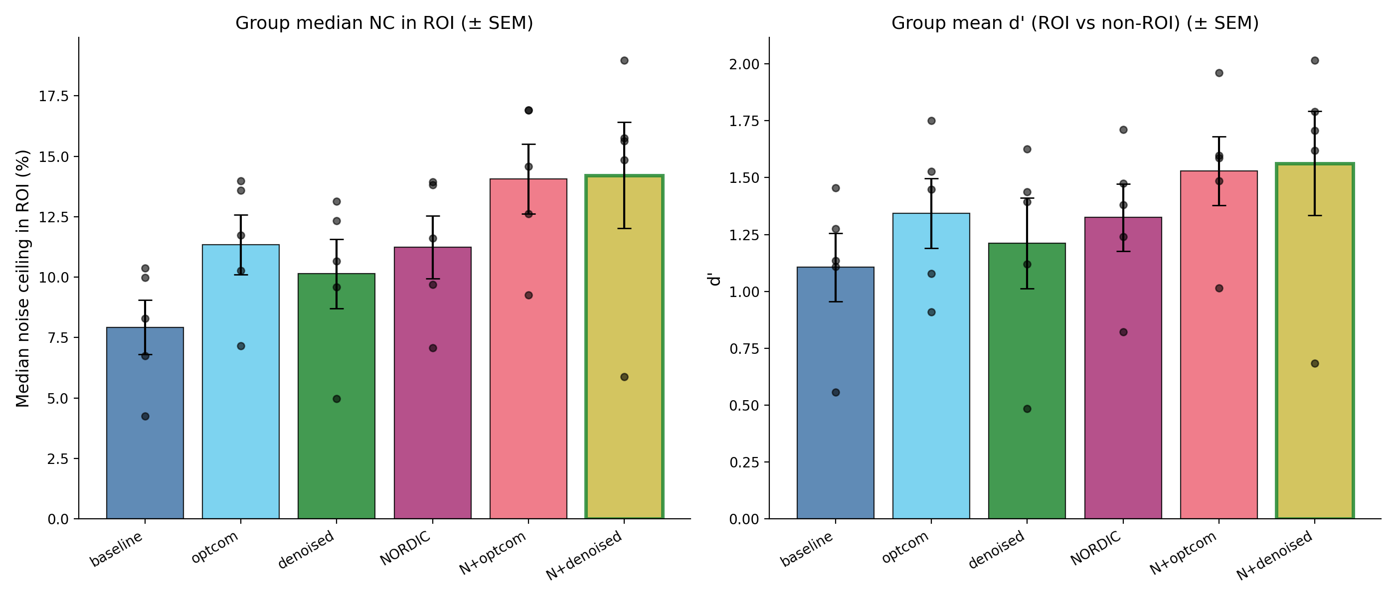
Preprocessing variant comparison for five subjects in ses-01. The left panel shows the median noise ceiling in visually responsive voxels; the right panel shows d-prime separation between visually responsive and non-responsive voxels. Points show individual subjects, and bars show group mean +/- SEM.

The comparison included sub-01, sub-03, sub-05, sub-06, and sub-07, with 12 runs per subject. NORDIC alone and tedana optcom alone gave similar improvements over the baseline preprocessing (about 42-43 % in median ROI noise ceiling). Combining NORDIC with tedana gave the largest gains, around 77-79 % in median ROI noise ceiling and 38-41 % in d-prime.

This result sits slightly outside the default GLMsingle advice. The GLMsingle documentation cautions that projecting out nuisance components before GLMsingle, including ICA-derived noise or low-rank approaches such as NORDIC, is not generally recommended because it can introduce bias and duplicate part of GLMsingle’s own data-driven denoising. In this dataset, NORDIC improved the noise-ceiling summaries, so we considered it justified despite the general caution.

We did not, however, choose the most aggressive variant. NORDIC followed by tedana ICA denoising was slightly ahead at the group level, but it reduced the noise ceiling for sub-07 relative to the NORDIC + optcom variant. Given that subject-specific drop, and because GLMsingle already performs its own GLMdenoise step, we picked NORDIC + tedana optcom for the beta pipeline. This keeps the gain from NORDIC while avoiding an additional ICA-denoising step that was not consistently beneficial across subjects.

A caveat is important here: this comparison used only one session, so the absolute noise-ceiling values are lower than they should be for the full dataset. Only stimuli with repeated presentations can enter the estimate, and most usable repeated stimuli in one session have only two presentations. However, this limitation applies equally to all six variants.

Output Files

See fMRI Data for a full description of the preprocessed output files, including confound regressors.

Quality Control

For quality control details - MRIQC metrics, motion thresholds, exclusion criteria, and known issues - see Quality Control.